Stress testing is a critical component of insurers’ enterprise risk management framework. Boards, managements, regulatory and rating agencies and other stakeholders have an expectation that organizations assess the “consequence of being wrong” in the formulation of their business strategies and the execution of operating plans.¹ There is the need to distinguish between the willingness to take risk and the capacity to absorb risk. The former is aspirational and can be reviewed in various constituent communications. The later becomes a fact proven only by the resiliency of the enterprise to recover from adverse events.

Insurers need to conduct stress tests for events having an impact on multiple facets of their businesses. Primarily, these would include insurance underwriting and investment activities. Additionally, insurers need to contemplate second-order events, such as extreme capital market outcomes occurring in the aftermath of adverse and sudden insurable events. The focus of this General ReView is investment stress testing. However, we do display historical underwriting results to place investment stress tests in context.

Investment stress testing can be performed several ways. One probabilistic approach is to rely upon an economic scenario generator to simulate a distribution of portfolio returns from which downside results can be assigned a probability of occurring.² A deterministic approach is to select particular historical events or periods of time to estimate the amount of loss if capital markets behaved similarly on a prospective basis. In either case, it is necessary to assess the plausibility of the stressed outcomes to avoid unwarranted actions.

Further, regardless of the methodology, the practitioner must decide some subtle but important timeline criteria. First, is the evaluation timeframe intra-period or end-of-period? Second, is the period of time monthly, quarterly or annually? Third, are losses accumulating over multiple years a consideration? Fourth, are losses defined on a marked-to-market basis?

Or, are only realized losses relevant? And finally, are taxes a consideration? Too frequently these criteria are not disclosed in stress testing regimes.

Our approach is to show pre-tax, marked-to-market outcomes for intra-period and end-of-period timeframes of differing time intervals. We apologize for the amount of data we show. However, the data is straightforward and it is often necessary to slough through the details to identify devilish consequences of overlooked intricacies in any approach. Hopefully, the information we show is useful to readers as they evaluate their own stress tests.

An Enterprise View of Stress

Chart 1 displays a 90-year history of U.S. property/casualty calendar year reported combined ratios and twenty-year fixed maturity U.S. government bond yields (GS 20-Yr.) against the background of U.S. business cycle contractions (BCC) as defined  by the National Bureau of Economic Research (NBER). The calendar year measure masks volatility of accident year results. However, it does reflect the impact of catastrophe losses.

Chart 1. U.S. Property/Casualty Combined Ratios and Government Bond Yields

In contrast to the volatility of underwriting results, investment yields appear tame, behaving more evolutionary than episodic. However, there are two caveats. First, changes in yield can translate into greatly amplified price and total return volatility. Second, year-end 2014 industry investment leverage (invest assets to capital) is about three times that of insurance leverage (premium to capital) so that a small amount of investment volatility can be as destabilizing to capital as fortuitously adverse underwriting results.

Periods of Worst Case Stress

We rely upon daily return data from 1962 (the earliest period of continuously available data) thru 2014 for the remainder of the exhibits. Table 1 below displays the five largest independent total return drawdowns occurring within a monthly and annual time interval on a rolling daily basis for a five year U.S. Treasury bond.

Table 1. Five-Year U.S. Government Maximum Total Return Drawdowns 1962–2014

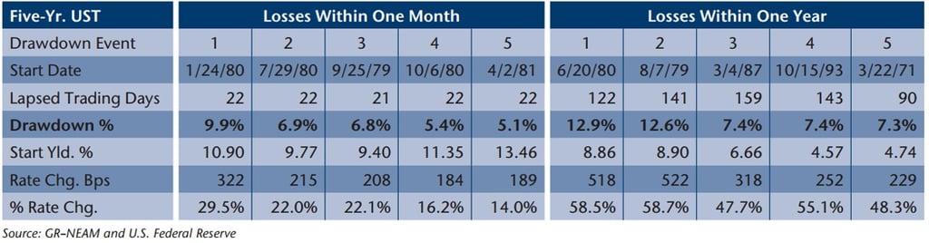
The seventies and early eighties are the dominant drawdown periods. In the case of a monthly time interval, all but one of the five largest drawdowns used the full 22 rolling trading days. On a one-year basis, the maximum drawdowns occurred as quickly as within 90 consecutive days and as slowly as within 159 days. Starting yields were very high in the most extreme drawdown periods, reflecting then current economic inflation. Note the largest drawdowns within the three- and five-year timeframes are the same as for the one-year (not shown).

In Table 2 we show the portfolio time periods having the greatest percentage rate change and the resulting drawdown and other statistics as shown above. The five largest monthly time interval percent rate change increases occurred after the recent “great recession” financial crisis and occasionally emerged within just a few days. However, the drawdowns were not large. On a one-year basis, the drawdowns were more significant but the securities redeemed at par, erasing the losses. Also, two of the annual time interval drawdown periods were well before the great recession.

Table 2. 5-Year U.S. Government Maximum Percent Rate Change 1962–2014

One month and one-year drawdowns for longer-duration and lower-rated securities were both more severe than shown above. Table 3 below displays drawdown results for 20-year BBB corporate bonds. The recent financial crisis plays more prominently in the one-month time horizon than the one-year time interval. Except for the fifth largest drawdown commencing October 28, 1993, the one-year time frame drawdowns are the same as those in the three- and five-year time intervals. Apart from events leading up to the Lehman default (2008), popular stress periods/financial calamities are not as untoward as those occurring in the 1970s and 1980s.

Table 3. 20-Year Corporate BBB Maximum Total Return Drawdowns 1962–2014

Table 4 focuses upon U.S. equities as proxied by the S&P 500 total return index. In contrast to fixed income, equity drawdowns are far more severe, lacking a coupon component to mute valuation volatility. Additionally, they continue to deteriorate for a more protracted period of time.

Table 4. S&P 500 Maximum Total Return Drawdowns 1962–2014

Table 5 displays stress outcomes across several asset categories. The upper portion

of the table shows drawdown statistics for BBB corporate bonds based upon the largest basis point spread widening time frames. The lower portion of the table displays the associated drawdown of 20-year constant maturity U.S. Treasury bonds and the S&P 500.

Table 5. Total Return Drawdowns Associated With Maximum Spread Widening 1962–2014

Within a monthly time interval, the 15 days beginning March 25, 1980 experienced the greatest spread widening in terms of basis point movement (210 bps). However, the value of the BBB bond actually appreciated (-0.2% drawdown), reflecting a decline in interest rates and a positive 17% total return of the 20-year U.S. Treasury bond (the rate proxy underlying BBB corporate yields). During the same period of spread widening, the total return of the S&P 500 was 2.4%. Unfortunately, the 22 days beginning September 25, 2008 were very unkind to both BBB corporate bonds (17.1%) and equities (29.8%).³

Conventional Historical Stress Events

In this section we focus upon several named event stress periods and business cycle contractions and their associated maximum drawdowns. The named events are not intended to be exhaustive but rather chosen to display the diversity of results among differing maturities and credit quality within fixed income and in contrast to equity valuations. These named events are frequently referenced by commercial vendors for stress testing.⁴

Table 6 displays the event specific results for the one-month and three-year time intervals. Note that the blank fields represent a net total return gain rather than a loss. The oil-related events of 1967 (King David’s War) and 1973 had an impact on all assets and had a multi-year effect. The 1979 energy crisis took a steep toll upon fixed income markets but not equity valuations.

Table 6. Maximum Total Return Drawdowns Associated With Name-Specific Events

The impact of the Lehman default was broad-based, sudden and severe (particularly for equities). Sovereign defaults (also associated with the Long-Term Capital Management debacle) had only a modest (immediate) adverse impact upon U.S. markets, often offset by the favorable impact of flight to quality (U.S. Treasury bonds). The Cuban Missile Crisis showed only fleeting impact within equity markets (for similar flight to quality reasons?).

Table 7 below shows similar information during periods of economic contraction and expansion for the U.S. economy, as defined by the NBER. The upper portion of the table displays drawdowns associated with periods of economic contraction. In general, other than for equity market valuations associated with the “great recession” beginning December 2007 and the “tech boom” downturn beginning in 2001, periods of economic contraction have been mild relative to those shown in prior tables.

Table 7. Maximum Total Return Drawdowns Associated with U.S. Economic Cycles

During all periods of economic contraction, fixed income drawdowns “maxed-out” within the first year’s anniversary of the start date. In the case of equities, the worst had passed within about 1.5 years (418 trading days in the case of the March 2001 downturn) from the start date. These timings roughly coincide to the NBER’s declaration of the downturns’ reversal. The uptick in fixed income and equity valuations is aligned with renewed economic activity. Recall that the NBER business cycle declarations are ex-post, not ex-ante. They are not prophetic and therein lies the linkage to the alignment.

The lower portion of Table 7 focuses upon periods of economic expansion. There are marked periods of fixed income and equity double-digit drawdowns. They coincide with the recovery beginning in 1980 (the most short lived of those recorded at 12 months) and during the early stages of recovery beginning in November 2001 following the tech boom contraction of March 2001. The later recovery lasted over six years.

Intra-Period Versus End-of-Period Losses

So far we have focused upon intra-period losses rather than those occurring during an end-of-period time frame. The advantage of the former is that they convey better a peak-to-trough drawdown as a measure of loss due to duress. Their disadvantage is that these periods of extreme drawdown do not coincide with fiscal (disclosure) periods. Relying upon end-of-period losses still requires decisions regarding the appropriate reporting period, for example, month-end versus quarter-end or year-end.

Table 8 displays the five largest month-end and year-end drawdowns (total return) over the period 1962–2014 for the four principal security proxies previously displayed. On a month-end basis, only three of the data points are associated with the recent financial crisis. On an annual basis, four of the data points occurred during the years of the crisis. Based upon a “data point count,” the decades preceding the most recent crisis were far more volatile. The question remains which is the “better” time-frame to capture market volatility?⁵

Table 8. Worst Monthly and Annual End-of-Period Loss 1962–2014

In contrast to the forgoing, Table 9 shows summary data based upon intra-period outcomes. The greatest significance of the two tables is the disparity between their estimates of maximum drawdowns: historic end-of period estimates mask the inherent underlying volatility of capital market total returns.

The second level of importance pertains to the approximate timing of the drawdown. On a monthly basis one-half the data points of the drawdown results are not at all similar as to approximate timing. Additionally, on an annual basis, only five are reasonably coincidental. Regardless of timeframe, the question remains, “Which is the “better” periodicity–monthly or annual–to estimate market volatility and its significance?”

Table 9. Maximum Monthly and Annual Intra-Period Drawdowns 1962–2014

Summary

Stress testing is a business best practice. Our interest in the topic is driven by the clients we serve. As we assist clients in managing their enterprise and investment risk, we are motivated to “get it right,” i.e., to assure a better understanding of the inherent risk within their insurance and investment portfolios. The following summarizes our thoughts in regard to historic scenario stress testing:

1. In contrast to insurance underwriting results, investment yield volatility appears tame—behaving more evolutionary than episodic. However, changes in fixed-income yields and spreads can translate into greatly amplified total return results. And, because investment leverage (assets-to-capital) is a multiple of insurance leverage (premium-to-capital), investment volatility can be as destabilizing to insurers’ capital as adverse underwriting results.
2. Some of the more “popular” stress events fail to offer a meaningful perspective

of potential downside loss. The reasons include that the events themselves had

little measurable impact; other unnamed “events” eclipsed their outcomes; and current market levels are not at all comparable to those associated with the periods

of greatest stress.⁶

3. Conventional wisdom is “in periods of stress, (all) asset valuations become highly correlated.” Credit-sensitive instruments do highly correlate with one another during “credit events” but high quality assets’ valuations might very well increase while lesser credits’ valuations’ might collapse and equity valuations are not bound to generalizations.
4. More conservative intra-period versus end-of-period time frames yield markedly different outcomes. The outcomes are different in two significant ways. First, the end-of-period estimates are a (small) fraction of intra-period losses. And second, the most severe drawdown dates for both monthly and annual time intervals are approximately the same for the two differing timeframes in less than one-half of

the cases.

5. Similarly, periodicity, monthly versus annual, greatly impacts the estimate of stress losses. Focusing on year-end valuations masks the possibility of ruinous outcomes at any time prior to that reporting period as well as at either end-of-month/quarter or intra-month/quarter. Conventional methods appear not to address these considerations and regulators and rating agencies provide mixed guidance.

We operate in an environment where we must make investment and other financial decisions using imperfect or incomplete information. Stress testing is one means to highlight areas where our decision making process might be weak, or even where opportunities might exist that we could otherwise overlook. As we consider ways to “stretch” our understanding of enterprise and investment risks, let’s be mindful of the reality of the past, understand its relevance to our future and not be subject to blind obedience to any method. The following link will take to you the full analysis: General Review.

Endnotes

1. McKinsey & Company, “Strategic insight through stress-testing: How to connect the ‘engine room’ to the boardroom,” July 2012. Corbet, Shaen., “The European Financial Market Stress Index,” Vol. 4, No.1, International Journal of Economic and Financial Issues. February, 2014. NAIC, “Own Risk and Solvency Assessment: Guidance Manual, July 2014., IMF, NAIC, EIOPA references. EIOPA.
2. We do not recommend economic scenario generators for several reasons. First, they are a “black box.” Second, their results from simulation to simulation cannot be replicated. And third, their calibration implies a degree of precision which does not exist in the context of the extreme events which are being tested.
3. We additionally address spread widening rather than only total return drawdowns in order to decompose the total return movement into interest rate and spread volatility. Also, recall a “positive” drawdown denotes a loss and a negative drawdown denotes a gain.
4. Most often the precise dates of the events are not provided and less frequently is the time horizon of the stress period specified.
5. We prefer intra-period time frames precisely because 1) they show a higher level of volatility than end-of-period results (we do want to understand “how bad it can be”), 2) adverse events only by happenstance coincide with calendar year-end fiscal reporting periods, and 3) peak-to-trough drawdowns might trigger other obligations such as loan covenants.
6. For example, the most severe intra-period short-term drawdown for the 5-year treasury exceeded 9.9% during the early 1980s when rates rose over 322 bps from starting levels of 10.90%. However, as a word of caution, a 322 bps rate increase from today’s levels would overwhelm the downside loss of the 1980s. The question one must ask concerns the circumstance or change to “the state of the world” that would precipitate such a move.